Kaggle テーブルデータコンペで使う EDA・特徴量エンジニアリングのスニペット集
随時追加していきます。間違いやもっとこうした方がいいなどあればコメントください。
前提
import pandas as pd
import multiprocessing
import numpy as np
import seaborn as sns
import sys
from itertools import chain
from collections import deque
import matplotlib.pyplot as plt
from pandas.io.json import json_normalize
import json
import warnings

train = pd.read_csv("../input/train.csv")
test = pd.read_csv("../input/test.csv")
EDA
データの確認
Notebook でデータを見る前に、コンペの Data > Data Description から、各データ・カラムの概要を理解する。場合によっては、csv でダウンロードして、スプレッドシートとして眺めてみる。
コンペデータのファイルを確認
!ls -GFlash /kaggle/input/<コンペ名称>/
例えば、2019 Data Science Bowl では、下記のように表示される。データの種類や、サイズなどを確認できる。
!ls -GFlash /kaggle/input/data-science-bowl-2019/

total 4.0G
4.0K drwxr-xr-x 2 root 4.0K Oct 23 16:22 ./
4.0K drwxr-xr-x 3 root 4.0K Oct 26 04:05 ../
 12K -rw-r--r-- 1 root  11K Oct 23 16:21 sample_submission.csv
400K -rw-r--r-- 1 root 400K Oct 23 16:21 specs.csv
380M -rw-r--r-- 1 root 380M Oct 23 16:22 test.csv
3.7G -rw-r--r-- 1 root 3.7G Oct 23 16:22 train.csv
1.1M -rw-r--r-- 1 root 1.1M Oct 23 16:21 train_labels.csv
データをランダムサンプリングする
1000000 レコードでランダムサンプリングする場合。データが大きすぎて、EDAでデータをプロットするのに時間がかかってしまう時などに利用する。
train_sampled = train.sample(1000000)
print(train.shape)
train_sampled = train.sample(1000000)
print(train_sampled.shape)
--------------
(11341042, 11)
(1000000, 11)
warningを表示しないようにする
warnings.filterwarnings('ignore')
データフレームの表示数を増やす
head 等で表示した際に省略されないようにする
pd.set_option('display.max_rows', None)
pd.set_option('display.max_columns', None)
pd.set_option("display.max_colwidth", 10000)
行数と列数を表示する
print("{} rows and {} features in train set".format(train.shape[0], train.shape[1]))
print("{} rows and {} features in test set".format(test.shape[0], test.shape[1]))
メモリ使用量を減らす
def reduce_mem_usage(df):
    start_mem = df.memory_usage().sum() / 1024**2
    print('Memory usage of dataframe is {:.2f} MB'.format(start_mem))

    for col in df.columns:
        col_type = df[col].dtype

        if col_type != object:
            c_min = df[col].min()
            c_max = df[col].max()
            if str(col_type)[:3] == 'int':
                if c_min > np.iinfo(np.int8).min and c_max < np.iinfo(np.int8).max:
                    df[col] = df[col].astype(np.int8)
                elif c_min > np.iinfo(np.int16).min and c_max < np.iinfo(np.int16).max:
                    df[col] = df[col].astype(np.int16)
                elif c_min > np.iinfo(np.int32).min and c_max < np.iinfo(np.int32).max:
                    df[col] = df[col].astype(np.int32)
                elif c_min > np.iinfo(np.int64).min and c_max < np.iinfo(np.int64).max:
                    df[col] = df[col].astype(np.int64)
            else:
                if c_min > np.finfo(np.float16).min and c_max < np.finfo(np.float16).max:
                    df[col] = df[col].astype(np.float16)
                elif c_min > np.finfo(np.float32).min and c_max < np.finfo(np.float32).max:
                    df[col] = df[col].astype(np.float32)
                else:
                    df[col] = df[col].astype(np.float64)
        else:
            df[col] = df[col].astype('category')

    end_mem = df.memory_usage().sum() / 1024**2
    print('Memory usage after optimization is: {:.2f} MB'.format(end_mem))
    print('Decreased by {:.1f}%'.format(100 * (start_mem - end_mem) / start_mem))

    return df
train = reduce_mem_usage(train)
test = reduce_mem_usage(test)
下記のように メモリ使用量 を最適化してくれる
Memory usage of dataframe is 1959.88 MB
Memory usage after optimization is: 530.08 MB
Decreased by 73.0%
Memory usage of dataframe is 1677.73 MB
Memory usage after optimization is: 462.08 MB
Decreased by 72.5%
並列処理でデータを read する
data ディレクトリにあるファイルをメモリ使用量を減らしつつ、並列処理でデータフレームとして読み込む。
path = "/kaggle/input/<コンペ名称>/"
data_list = glob(path + '*.csv')

def load_data(data):
    return reduce_mem_usage(pd.read_csv(data))

with multiprocessing.Pool() as pool:
    sample, test, train = pool.map(load_data, data_list)
pandas 基本
train.dtypes
train.info()
train['col_name'].value_counts()
train.shape
train.columns
train.query('col_name < 0')
train['col_name'].unique()
train.drop_duplicates()
train.isna()
カラムごとのユニーク数とユニーク値の表示
for col, values in train.iteritems():
    num_uniques = values.nunique()
    print ('{name}: {num_unique}'.format(name=col, num_unique=num_uniques))
    print (values.unique())
    print ('\n')
統計量の表示
カラム名 / カラムごとのユニーク値数 / 最も出現頻度の高い値 / 最も出現頻度の高い値の出現回数 / 欠損損値の割合 / 最も多いカテゴリの割合 / dtypes を表示する。
%%time
stats = []
for col in train.columns:
    stats.append((col,
                  train[col].nunique(),
                  train[col].value_counts().index[0],
                  train[col].value_counts().values[0],
                  train[col].isnull().sum() * 100 / train.shape[0],
                  train[col].value_counts(normalize=True, dropna=False).values[0] * 100,
                  train[col].dtype))
stats_df = pd.DataFrame(stats, columns=['Feature', 'Unique values', 'Most frequent item', 'Freuquence of most frequent item', 'Percentage of missing values', 'Percentage of values in the biggest category', 'Type'])
stats_df.sort_values('Percentage of missing values', ascending=False)
例えば、2019 Data Science Bowl では、下記のように表示される。
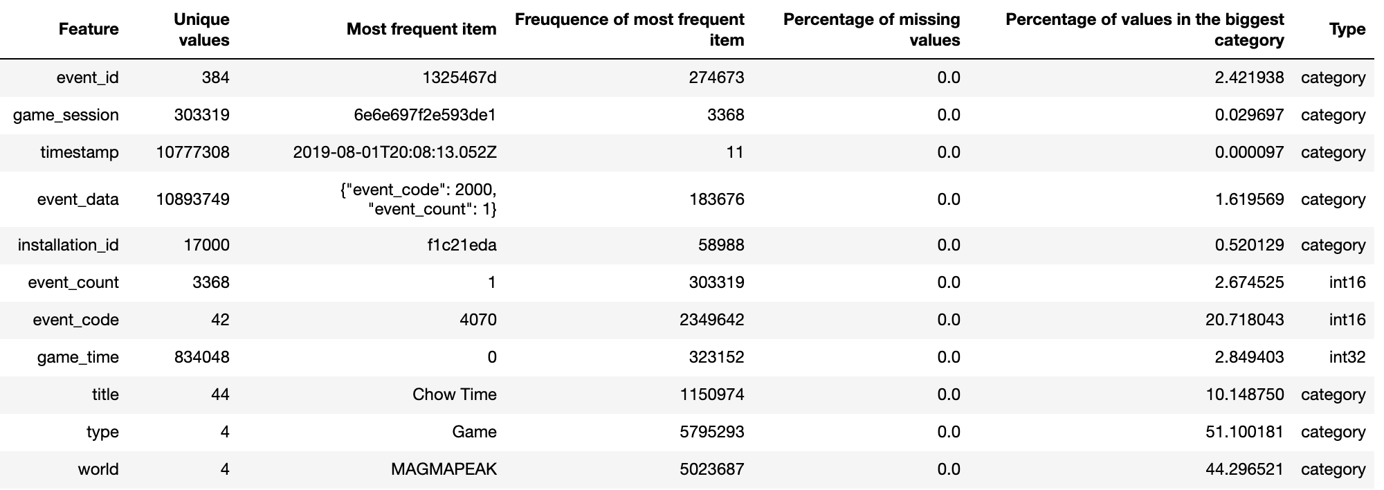
参考:https://www.kaggle.com/artgor/is-this-malware-eda-fe-and-lgb-updated
全カラムのヒストグラム表示
train.hist(bins=50, figsize=(80,60))
plt.show()
特定のカラムのヒストグラム表示
train['col_name'].plot(kind='hist', bins=200, figsize=(15, 5), title='Distribution of col_name')
# log scaleの場合
train['col_name'].apply(np.log).plot(kind='hist', bins=200, figsize=(15, 5), title='Distribution of col_name')
plt.show()
2値分類タスクで target のカテゴリごとに特定のカラムのヒストグラムを表示
log scale した場合
fig, (ax1, ax2) = plt.subplots(2, figsize=(15, 6))
train[train['target'] == 1]['col_name'].apply(np.log).plot(kind='hist', bins=100, title='Log col name - 1', color='#348ABD', xlim=(-3, 10), ax=ax1)
train[train['targe'] == 0]['col_name'].apply(np.log).plot(kind='hist', bins=100, title='Log col name - 0', color='#348ABD', xlim=(-3, 10), ax=ax2)
plt.show()
散布図
plt.figure(figsize=(15, 5))
plt.scatter(train['x_cols'], train['y_cols'])
plt.title('title')
plt.xlabel('x_col_name')
plt.ylabel('y_col_name')
plt.show()
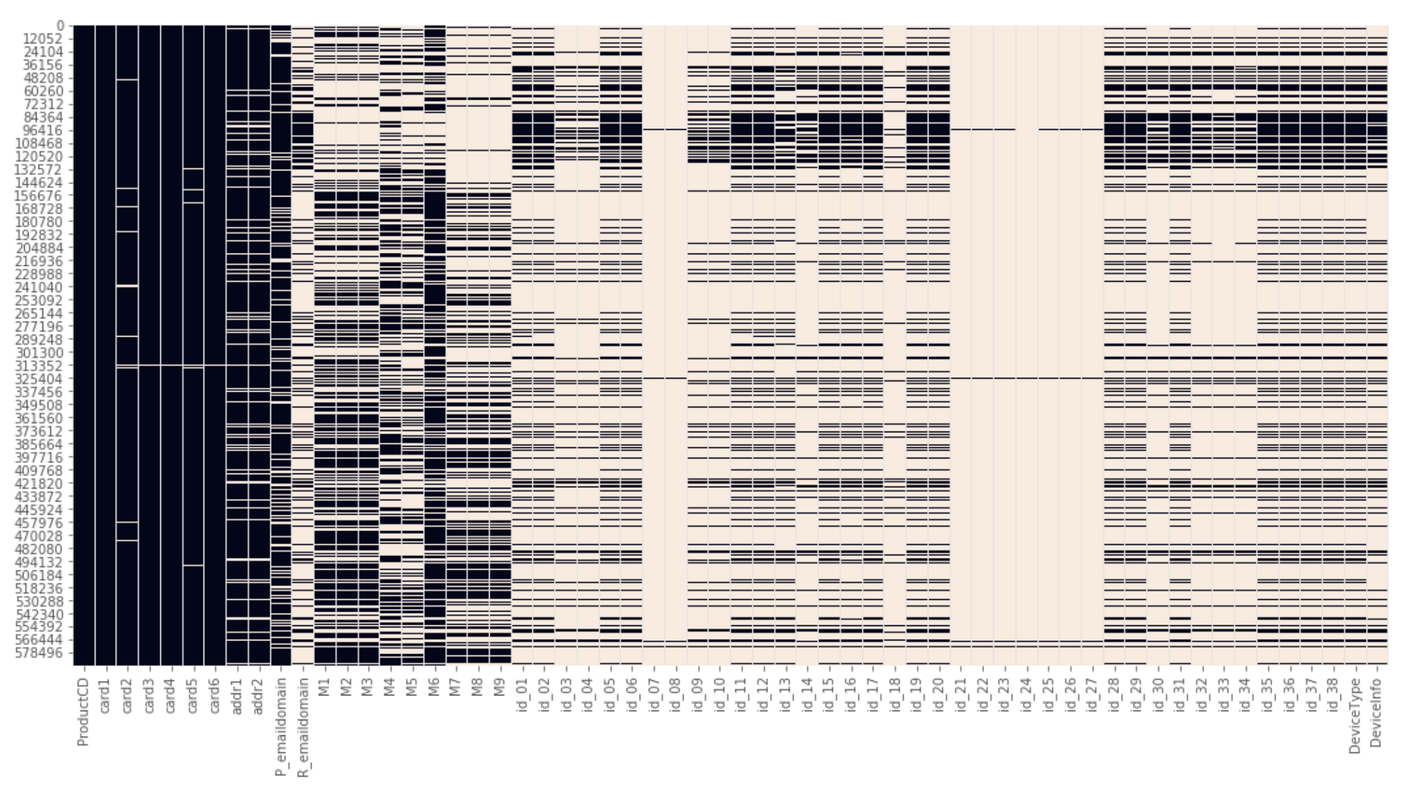
欠損値をヒートマップで視覚化
データ全体における欠損値を概要を理解する
plt.figure(figsize=(18,9))
sns.heatmap(train.isnull(), cbar=False)
欠損している箇所が白く表示されるため、全体としてどのようにデータが欠損しているか理解できる。 参考:https://www.kaggle.com/suoires1/fraud-detection-eda-and-modeling より
特徴量同士の相関をヒートマップで表示
fig, ax = plt.subplots(figsize=(12, 9))
sns.heatmap(train.corr(), square=True, vmax=1, vmin=-1, center=0)
ターゲットとその他の特徴量との相関
train.corr()['target'].sort_values()
分類タスクにおけるターゲット変数の割合
train['target'].value_counts()
変数のメモリ使用量を表示する
def compute_object_size(o, handlers={}):
    dict_handler = lambda d: chain.from_iterable(d.items())
    all_handlers = {tuple: iter,
                    list: iter,
                    deque: iter,
                    dict: dict_handler,
                    set: iter,
                    frozenset: iter,
                   }
    all_handlers.update(handlers)     # user handlers take precedence
    seen = set()                      # track which object id's have already been seen
    default_size = sys.getsizeof(0)       # estimate sizeof object without __sizeof__

    def sizeof(o):
        if id(o) in seen:       # do not double count the same object
            return 0
        seen.add(id(o))
        s = sys.getsizeof(o, default_size)

        for typ, handler in all_handlers.items():
            if isinstance(o, typ):
                s += sum(map(sizeof, handler(o)))
                break
        return s

    return sizeof(o)

def show_objects_size(threshold, unit=2):
    disp_unit = {0: 'bites', 1: 'KB', 2: 'MB', 3: 'GB'}
    globals_copy = globals().copy()
    for object_name in globals_copy.keys():
        size = compute_object_size(eval(object_name))
        if size > threshold:
            print('{:<15}{:.3f} {}'.format(object_name, size, disp_unit[unit]))

# 100MB超のオブジェクト一覧を表示する
show_objects_size(100)
参考:https://qiita.com/nannoki/items/1466779987b68c4f4bf9
データのカラムリストから 特定のカラムを取り除いたリストを取得する
drop_cols = ['a', 'b', 'c', 'd', 'e'] # 取り除きたいカラムのリスト
cols = [c for c in train.columns if c not in drop_cols]
データフレームへの処理の並列化
def df_parallelize_run(df, func):
    num_partitions, num_cores = psutil.cpu_count(), psutil.cpu_count()
    df_split = np.array_split(df, num_partitions)
    pool = multiprocessing.Pool(num_cores)
    df = pd.concat(pool.map(func, df_split))
    pool.close()
    pool.join()
    return df
特徴量エンジニアリング
特定の文字を含んだカラム名のリストを得る
# 'target' という文字を含んだカラムを取得
cols = [c for c in train.columns if 'target' in str(c)]
json 形式のカラムを複数のカラムに展開する
df_json = json_normalize(train['json_col'].apply(lambda x: json.loads(x)))
複数の情報を含んだカラムを分割する
Android 6.0.1、iOS 11.4.0 といった OSとバージョン情報を複数含んだカラムを分割する。
# アンダーバーで分割
train['OS'] = train['OS_VERSION'].str.split('_', expand=True)[0]
train['VERSION'] = train['OS_VERSION'].str.split('_', expand=True)[1]
Count Encoding
カテゴリ変数の列で各カテゴリの出現回数をカウント。ここでは、train と test における出現回数を合計した特徴量を生成。カテゴリ値の人気度を測定しているようなものと解釈する。 参考:https://blog.datarobot.com/jp/automatedfeatureengineering
train['col_name_count'] = train['col_name'].map(pd.concat([train['col_name'], test['col_name']], ignore_index=True).value_counts(dropna=False))
test['col_name_count'] = test['col_name'].map(pd.concat([train['col_name'], test['col_name']], ignore_index=True).value_counts(dropna=False))
clipping
# 99%
upperbound, lowerbound = np.percentile(train['col_name'], [1, 99])
train['col_name_clipped'] = np.clip(train['col_name'], upperbound, lowerbound)
normalize
train['col_name_nomalize'] = (train['col_name'] - train['col_name'].mean() ) / train['col_name'].std()
カテゴリ変数のみ Label Eoncoding する
from sklearn.preprocessing import LabelEncoder

for col in train.columns:
    if train[col].dtype == 'object':
        le = LabelEncoder()
        le.fit(list(train[col].astype(str).values) + list(test[col].astype(str).values))
        train[col] = le.transform(list(train[col].astype(str).values))
        test[col] = le.transform(list(test[col].astype(str).values))
行のNAN数を新しい特徴量に
train['number_of_NAN'] = train.isna().sum(axis=1).astype(np.int8)
ビニング処理
ビンに含まれる個数を指定
df['col_name_qcut_10'] = pd.qcut(df['col_name'], 10)
test データに無い場合1、ある場合は0にする特徴量
train['col_name_check'] = np.where(train['col_name'].isin(test['col_name']), 1, 0)
# test の場合は逆
test['col_name_check']  = np.where(test['col_name'].isin(train['col_name']), 1, 0)
全て0のカラムを作成する
train["col_name_zero"] = np.zeros(train.shape[0])
NaN とそれ以外の値の特徴量を作成する
train['col_name_nan'] = np.where(train['col_name'].isna(), 1, 0)
nan 数の同じカラムごとにグループ化
nans_groups = {}
nans = pd.concat([train, test]).isna()

for col in train.columns:
    cur_group = nans[col].sum()
    if cur_group > 0:
        try:
            nans_groups[cur_group].append(col)
        except:
            nans_groups[cur_group] = [col]

for n_group, n_members in nans_groups.items():
    print(n_group, len(n_members), n_members)
Aggregated Features
カテゴリのグループごとに aggregation する。例えば、同じip, os, deviceの総クリック数を計算するなど。参考:Kaggle Masterに学ぶ実践的機械学習[Kaggle TalkingData Competition編]
agg_types = ['max', 'min', 'sum', 'mean', 'std', 'count']
for agg_type in agg_types:
    new_col_name = cat_col + '_' + agg_col + '_' + agg_type
    temp = pd.concat([train[[cat_col, agg_col]], test[[cat_col, agg_col]]])
    temp = temp.groupby([cat_col])[agg_col].agg([agg_type]).reset_index().rename(columns={agg_type: new_col_name})
    temp.index = list(temp[cat_col])
    temp = temp[new_col_name].to_dict()
    train[new_col_name] = train[cat_col].map(temp)
    test[new_col_name]  = test[cat_col].map(temp)
numeric feature を 0以上にシフトする
for col in train.columns:
    if not ((np.str(train[col].dtype)=='category')|(train[col].dtype=='object')):
        min = np.min((train[col].min(), test[col].min()))
        train[col] -= np.float32(min)
        test[col] -= np.float32(min)
numeric feature の 欠損値を -1 で埋める
for col in train.columns:
    if not ((np.str(train[col].dtype)=='category')|(train[col].dtype=='object')):
        train[col].fillna(-1, inplace=True)
        test[col].fillna(-1, inplace=True)
frequency encoding
カテゴリ変数の出現回数で変数を置き換える。
def freq_enc(train, test, cols):
    for col in cols:
        df = pd.concat([train[col], test[col]])
        vc = df.value_counts(dropna=True, normalize=True).to_dict()
        vc[-1] = -1 # 欠損値を -1 で埋める場合
        new_col = col + '_freq_enc'
        train[new_col] = train[col].map(vc)
        train[new_col] = train[new_col].astype('float32')
        test[new_col] = test[col].map(vc)
        test[new_col] = test[new_col].astype('float32')

freq_enc(train, test, feature_list)
特徴量同士を結合した特徴量を作成し Label Encoding
def conb_enc(col1, col2, train, test):
    nm = col1 + '_' + col2
    train[new_col] = train[col1].astype(str) + '_' + train[col2].astype(str)
    test[new_col] = test[col1].astype(str) + '_' + test[col2].astype(str)
    le = LabelEncoder()
    le.fit(list(train[new_col].astype(str).values) + list(test[new_col].astype(str).values))
    train[new_col] = le.transform(list(train[new_col].astype(str).values))
    test[new_col] = le.transform(list(test[new_col].astype(str).values))
あるカラム群の欠損の数の合計を特徴量にする
train['missing'] = train[col_list].isna().sum(axis=1).astype('int16')
test['missing'] = test[col_list].isna().sum(axis=1).astype('int16')
特徴選択
constant なカラムを抜き出す
90%以上、同じ値のカラムを抜き出す
def get_constant_cols(df):
    constant_cols = [col for col in df.columns if df[col].value_counts(dropna=False, normalize=True).values[0] > 0.9]
    return constant_cols

cols = get_constant_cols(train)
不要なカラムを落とす
- 値が一つしかないカラム
- null が多いカラム
- ほとんど同じ値のカラム
one_value_cols = [col for col in train.columns if train[col].nunique() <= 1]
one_value_cols_test = [col for col in test.columns if test[col].nunique() <= 1]

many_null_cols = [col for col in train.columns if train[col].isnull().sum() / train.shape[0] > 0.9]
many_null_cols_test = [col for col in test.columns if test[col].isnull().sum() / test.shape[0] > 0.9]

big_top_value_cols = [col for col in train.columns if train[col].value_counts(dropna=False, normalize=True).values[0] > 0.9]
big_top_value_cols_test = [col for col in test.columns if test[col].value_counts(dropna=False, normalize=True).values[0] > 0.9]

cols_to_drop = list(set(many_null_cols + many_null_cols_test + big_top_value_cols + big_top_value_cols_test + one_value_cols+ one_value_cols_test))

train.drop(cols_to_drop, axis=1, inplace=True)
test.drop(cols_to_drop, axis=1, inplace=True)
再帰的特徴量選択
from sklearn.feature_selection import RFE
from sklearn.ensemble import RandomForestClassifier

X_train = train.drop('target', axis=1)
y_train = train['target']

select = RFE(RandomForestClassifier(n_estimators=100, random_state=42), n_features_to_select=40)
select.fit(X_train, y_train)

X_train_rfe = select.transform(X_train)
X_test_rfe = select.transform(test)
コルモゴロフ-スミルノフ検定を利用した特徴量選択
from scipy.stats import ks_2samp
list_p_value =[]

for i in tqdm(train.columns):
    list_p_value.append(ks_2samp(test[i], train[i])[1])

Se = pd.Series(list_p_value, index=train.columns).sort_values()
list_discarded = list(Se[Se < .1].index)
参考:https://www.kaggle.com/c/elo-merchant-category-recommendation/discussion/77537
Null Importance による特徴量選択
LightGBM などの学習器における feature importance で、上位に来た特徴量の中にノイズになっているものが含まれていることがある。そこで正しい目的変数で学習した結果の feature importance と目的変数を shuffle したデータを用いて学習した結果の feature importance を比較することでノイズになっている特徴量を抽出する。
def get_feature_importances(X, shuffle, seed=None):
    cols_to_drop = ['col_to_drop_1','col_to_drop_2']
    categoricals = ['cat_col']
    y = X['target']
    X = X.drop(cols_to_drop, axis=1)

    if shuffle:
        y = np.random.permutation(y)

    train = lgb.Dataset(X, y, free_raw_data=False, silent=True)

    lgb_params = {
        'objective': 'binary',
        'boosting_type': 'rf',
        'subsample': 0.623,
        'colsample_bytree': 0.7,
        'num_leaves': 127,
        'max_depth': 8,
        'seed': 42,
        'bagging_freq': 1,
        'n_jobs': 4
    }

    clf = lgb.train(params=lgb_params, train_set=train, num_boost_round=200, categorical_feature=categoricals)

    df_importance = pd.DataFrame()
    df_importance["feature"] = list(X.columns)
    df_importance["importance"] = clf.feature_importance()
    df_importance['train_score'] = roc_auc_score(y, clf.predict(X)) # 二値分類の場合

    return df_importance

def display_distributions(df_actual_importance, df_null_importance, feature):
    actual_imp = df_actual_importance.query(f"feature == '{feature}'")["importance"].mean()
    null_imp = df_null_importance.query(f"feature == '{feature}'")["importance"]

    fig, ax = plt.subplots(1, 1, figsize=(6, 4))
    a = ax.hist(null_imp, label="Null importances")
    ax.vlines(x=actual_imp, ymin=0, ymax=np.max(a[0]), color='r', linewidth=10, label='Real Target')
    ax.legend(loc="upper right")
    ax.set_title(f"Importance of {feature.upper()}", fontweight='bold')
    plt.xlabel(f"Null Importance Distribution for {feature.upper()}")
    plt.ylabel("Importance")
    plt.show()

# 実際の目的変数で学習し、feature importance の DataFrame を作成
df_actual_importance = get_feature_importances(X=reduce_train, shuffle=False)

# シャッフルした目的変数で学習し、feature importance の DataFrame を作成
nb_runs = 100
df_null_importance = pd.DataFrame()
for i in range(nb_runs):
    df_importance = get_feature_importances(X=reduce_train, shuffle=True)
    df_importance["run"] = i + 1
    df_null_importance = pd.concat([df_null_importance, df_importance])

# 実データにおいて特徴量の重要度が高かった上位5位を表示
for feature in actual_imp_df["feature"][:5]:
    display_distributions(df_actual_importance, df_null_importance, feature)

# 閾値を設定
THRESHOLD = 80

# 閾値以下(ノイズ)の特徴量を取得
not_important_features = []
for feature in df_actual_importance["feature"]:
    actual_value = df_actual_importance.query(f"feature=='{feature}'")["importance_split"].values
    null_value = df_null_importance.query(f"feature=='{feature}'")["importance_split"].values
    percentage = (null_value < actual_value).sum() / null_value.size * 100
    if percentage < THRESHOLD:
        not_important_features.append(feature)
参考